Resetting Expectations for the Rates of Natural Source Zone Depletion

Natural Source Zone Depletion (NSZD) is a term used for the mass loss of LNAPL contaminants in the subsurface due to a combination of processes. NSZD has become a buzzword associated with petroleum releases and is increasingly proposed as a final remedy for contaminated sites. Additionally, measured NSZD rates are used to shut down treatment systems that perform poorly. However, readers must be cautioned. The magnitude of the measured NSZD rates can change depending on critical method implementation details. Hence, the accuracy of the results can vary.
This article describes the evolution of the measurement of NSZD rates by surficial CO2 flux using passive traps. This evolution has led to NSZD rates that are more accurate and significantly lower than earlier estimates. The ranges of reported NSZD rates from different sources vary considerably because of the technique evolution. Based on early reports, an industry wide value of 1,000 gallons annually per acre of LNAPL losses was thought to be common. Practices developed over the last decade to control measurement error result in median measured values of 200 gallons/acre/year – while measured rate values of 1,000 gallons/acre/year are still occasionally obtained with the more recent practices, they are relatively uncommon. A “one size fits all” range should not be expected before performing the measurements.
Introduction: NSZD and Methods to Measure NSZD Rates
A fundamental concept of NSZD is that degradation of petroleum contaminants (mostly due to microbial activity) results in the production of biogas, a mixture of carbon dioxide (CO2) and methane (see Figure 1). These gases are more easily monitored in the unsaturated zone than in groundwater. While CO2 is stable, methane is not — it is readily transformed by aerobic microbes into CO2 once it migrates to shallow depths and encounters ambient O2.
Measured NSZD rates obtained using the multiple methods available have been compiled (Garg et al., 2017; Kulkarni et al., 2022). These compilations show median ranges around 1,000 to 2,000 gallons/acre/year. Based on these compilations, a “common knowledge” average of 1,000 gallons/acre/year has become an unwritten rule for NSZD. Because the magnitude of the measured ranges can have a strong impact on the LNAPL conceptual site model (e.g., see DiMarzio and Zimbron, 2019), these published ranges have generated an industry-wide expectation.
The goal of this article is to alert the reader that the common knowledge ranges are based on early NSZD rate measurement work using the first version of the passive CO2 flux traps. This technique has been improved over the years. The latest improvements show that the median value is in the order of 200 gallons/acre/year, much lower than the 1,000-2,000 gallons/acre/year or higher measured using the first version. In the next section, the method changes associated with each version and their impact on the measured values will be discussed.
Conceptually, a direct NSZD rate measurement would require two independent measurements of the contaminant mass at different times: the difference between both mass measurements, divided by the elapsed time would result in mass losses. This conceptually simple approach is impractical because: a) the methods to measure source mass are expensive; b) these methods have uncertainty (it is easy to miss part of the contamination); and c) a time required for significant contaminant mass losses might be impractically long (i.e., decades).
Fortunately, short term expressions of contaminant mass losses can be measured, and they constitute the base of indirect NSZD rate measurements. These methods assume a reaction and rely on measuring the production rate of the reaction products (for example, CO2 or heat, measured using a mass or a heat balance, respectively), which is then converted to contaminant losses on a per footprint area and time basis (for example, gallons of contaminant per acre per year).
The compositional method is one additional method based on changes in composition of the remaining LNAPL, which provides relative mass losses for individual compounds with respect to others (Hostettler et al., 2013). These methods are included in multiple guidance documents (API, 2017; ITRC, 2018; CRCCare, 2018; ASTM, 2022, among others). These documents typically describe the rationale of the methods, case studies, example calculations, and results from different methods.
All the byproducts used in the methods are naturally produced by soils, so it is essential to distinguish between a source not related to contamination (“natural”) and a source from petroleum contaminants. In other words, it is critical to separate the signal from NSZD and the noise (from sources not related to NSZD). For example, CO2 is produced by non-contaminated soils through the natural carbon cycle. Processes not associated with contamination are known as background processes. Some techniques rely on measuring the signal used to calculate NSZD rates (i.e., CO2 production rate) at one or more non-contaminated (background) locations. A background location correction means that the measured rate at one or more background locations is subtracted from measurements at contaminated locations.
Some methods do not require this background location correction. For example, a radiocarbon correction can be applied to surface CO2 flux-based methods. The radiocarbon (14C) composition of ancient carbon (including petroleum) is vastly different from ambient carbon (modern carbon). Modern sources are radiocarbon rich (with similar 14C levels to atmospheric values, where it is produced due to the action of cosmic rays). Because 14C is unstable (its self-decay half-life is ~ 6,000 years), samples older than ~ 60,000 years (i.e., petroleum) are completely depleted of 14C. The 14C correction is location specific, while the background correction assumes a constant site-wide value.
The Evolution of the Passive CO2 Trap Method
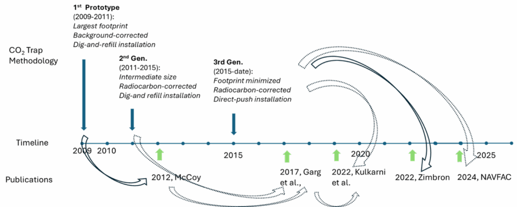
Colorado State University developed and validated the passive CO2 trap method using column soil experiments starting in 2009. A prototype was then tested at multiple sites (McCoy, 2012). The method was licensed to E-Flux in 2012. The hardware design, the installation method, and the correction applied to differentiate between CO2 from NSZD and naturally produced CO2 in soils evolved as follows:
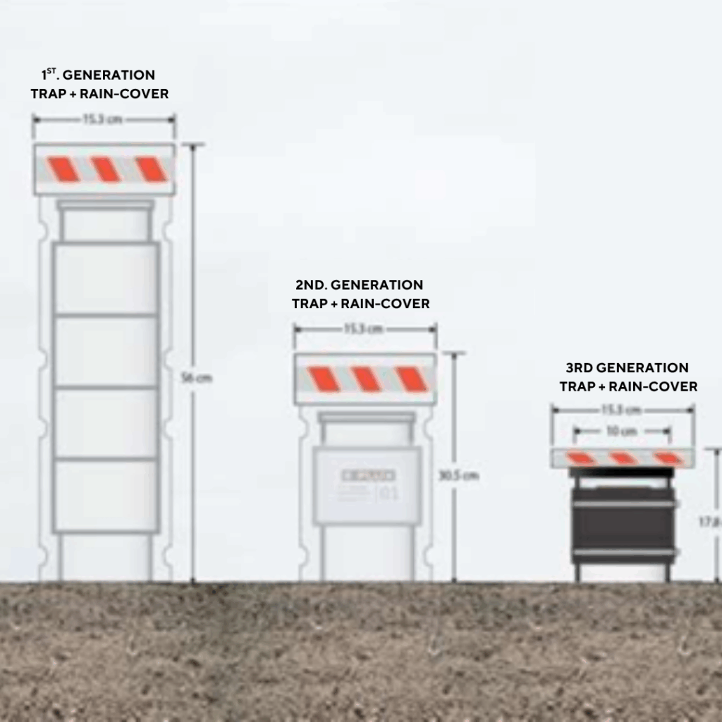
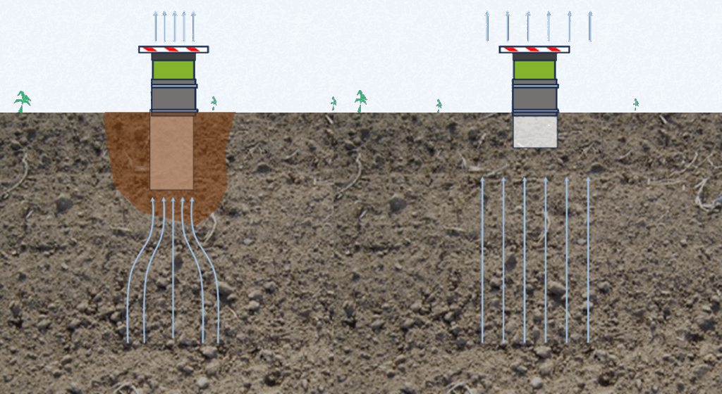
- First-generation CO2 traps (used from 2009 to approximately 2011). This first prototype provided proof of concept data (McCoy, 2012). The trap was approximately 20 inches tall, with a 6-inch tubular rain cover. NSZD rates were calculated using the background correction technique (instead of the 14C-correction). Figure 2 shows this design in comparison with the ones that followed. Most first-generation installations were done with the dig-and-refill method, in which the soil receiver was installed in a pre-dug hole, with the excavated soil used to refill the void, and then compacted back to the original soil conditions (see Figure 3). Note this last practice was part of the original protocols included in the API guidance document (API, 2017).
- Second-generation CO2 traps (used from 2011-2015). The height was ~ 12 inches, with a 6-inch OD tube rain cover. Some projects that used this design continued to use the 20-inch tall rain cover from the previous design. Additionally, some of these projects might have used the dig-and-refill receiver installation, but that practice was discouraged after 2011 as there was evidence that this caused a high bias (Goodwin and Palaia, 2011). Instead, the standard recommendation was to push the receiver directly into the soil to a depth of about 1 inch. Figure 3 illustrates the relative preferential flow effects caused by the soil disturbance of the dig-and-refill method.
- Third-generation CO2 traps (used since 05/2015 to date). This version was designed to minimize high bias due to high wind smokestack (Venturi) effects (Tracy, 2013; E-Flux, 2015). The height was 7 inches, with a flat rain cover (rather than a tube) to minimize the lateral profile. All values using this last generation design were 14C-corrected. A reinstallation at a field site replacing the first-generation design (installed with dig-and-refill method) with the direct-push installation of the third-generation design resulted in a reduction of 90% in the 14C-corrected measured values (one order of magnitude) (CDPHE, 2015).
The Sources of Reported NSZD Ranges
The reported ranges of field-measured NSZD rates from multiple sources are summarized in Figure 4. These sources include:
- McCoy, 2012. This work laid the initial development of the passive CO2 traps, including laboratory validation and data from five sites using a first-generation design. The NSZD values were background-corrected, not radiocarbon (14C) corrected. Locations with total CO2 fluxes equal or smaller than a clean background location (if available) were not reported.
- Garg et al., 2017. This overview included a description of the mechanisms related to NSZD, a summary of reported rates using multiple methods at a total of 25 NAPL sites, as well as potential factors controlling the mechanisms. The sites included those reported in the McCoy, 2012 and Piontek, et al., 2015 references.
- Kulkarni et al., 2022. This study collected NSZD rates using multiple methods from 40 LNAPL sites, and looked at correlations between fuel type, methods used, and seasonal and multi-year trends for sites with available data.
- Zimbron, 2022. This work compared two different corrections for the total CO2 flux raw using the CO2 traps, one using radiocarbon (14C) analysis, and a second using the background location correction for total CO2 flux. All these values were obtained using the third- and current generation of the CO2 traps, used since 2015 to minimize concerns about wind effects caused by the large size and footprint of previous versions (E-Flux, 2015).
- NAVFAC, 2024. The Naval Facilities Engineering Systems Command (NAVFAC) recently conducted NSZD measurements at five sites, all with the third generation CO2 trap, reporting average site-wide values, rather than individual measurements. This report included measurements using other techniques.
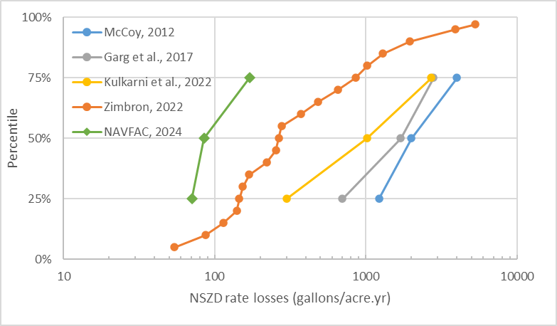
Figure 5 helps visualize how the data set for each of the literature sources compares to the other. This might be better illustrated by assuming how a hypothetical site falls in these ranges. For example, a site with a measured NSZD rate of 265 gallons/acre/year would exceed about 50% of the measured values in the Zimbron, 2022 data set, but would only exceed about 25% of the values in the Kulkarni et al. (2022) data set. A site with a measured NSZD rate of 1,000 gallons/acre/year would be in the middle (the median) of the Kulkarni et al. (2022) dataset, but would exceed 80% of the values in the Zimbron (2022) dataset.
Why Are Different Sources of NSZD Rates Inconsistent With Each Other?
The different NSZD rate measurement methods were based on first principles (i.e., laws of nature), using seemingly reasonable assumptions (e.g., one-dimensional gas flow). Some methods were further validated in laboratory studies (e.g., the CO2 trap-measured fluxes were compared against actual fluxes on a large soil column, see McCoy, 2012). Field applications were expected to include site variability (either between locations, or temporary soil conditions) – as a result, field measurements were expected to be an “order of magnitude estimate” (API, 2017). When trying to compare different methods in the field, or while repeating measurements on the same site using the same method, large differences (100%, equivalent to 2x, or higher) were expected.
The Kulkarni et al. (2022) and the Garg et al. (2017) compilations mentioned above provided similar ranges between the 25 and 75 percentile values, with the Kulkarni et al. (2022) report showing values two times smaller than those of Garg et al. (2017), at the lower range (and very similar values at the upper range, i.e., the 75 percentile). However, the data set from Zimbron (2022) shows a range approximately one order of magnitude smaller (the values are ~10x smaller) than the two above-mentioned compilations, whereas the data set from McCoy (2012) shows a range with larger values than the two compilations mentioned.
The McCoy (2012) and the Zimbron (2022) data sets were obtained with a similar instrument (passive CO2 traps) – however, the differences in the trap design, the installation, and the 14C correction resulted in much lower values associated with the last CO2 trap version. The original sources for CO2 trap data used in the Garg et al. (2017) and Kulkarni et al. (2022) compilations included data from either background-corrected first-generation CO2 traps (McCoy, 2012) and/or 14C-corrected values obtained with second-generation traps (e.g., Goodwin and Palaia, 2014). The reported values of the five sites included in the NAVFAC Fact Sheet (2024) (obtained with the last generation CO2 trap design and its updated recommended practices) are even lower than those of the Zimbron (2022) data set.
The Zimbron (2022) data set included only five sites, whereas the Garg et al. (2017) and Kulkarni, et al. (2022) reports included larger data sets (25 and 40 sites, respectively). The Zimbron (2022) data set was used because these data sets were publicly available (non-confidential), and the measurements included total CO2 fluxes in addition to the radiocarbon corrected (or fossil fuel) CO2 fluxes used to calculate NSZD rates. The two values (total CO2 and 14C-corrected CO2) allowed a comparison of both corrections (14C and background location). The E-Flux historical database comprising hundreds of sites measured since 2015 (not shown in Figure 4 to preserve the confidentiality of the data), includes values of the 14C-corrected NSZD rates even smaller than those in the Zimbron (2022) report.
Background corrected values had relatively poor correlations against the more rigorous 14C-corrected values (Zimbron, 2022). The two corrections agreed with each other in only one of the five sites included. Although other sites showed correlations between the results of both corrections, these vary among the different sites. More importantly, these correlations often resulted in higher average values for the background corrected NSZD rates than the 14C-corrected NSZD rates. The current standard approach for the passive CO2 traps is to apply the 14C-correction to multi-day deployment time integrated CO2 fluxes – error propagation techniques suggest that a typical detection limit equivalent to ~30 gallons/acre per year (the detection limit for each batch of samples is calculated based on the variability of the total and 14C analyses conducted).
The importance of the range of NSZD rate measurement values might be put in perspective by comparing NSZD data with other systems associated with gas phase biodegradation products. For example, Garg et al. (2017) referenced degradation rates in similar units (gallons/acre/year) for methane digesters, wetlands, landfills, and LNAPL NSZD sites (among others). LNAPL contaminated sites studied for vapor intrusion (VI) offer the same problem analyzed with similar tools from a different point of view. Lahvis et al. (1999) analyzed a gasoline spill in Beaufort, South Carolina. The reported biodegradation rates for individual gasoline components based on gas transport-based rates were equivalent to 180-830 gallons/acre/year. A similar analysis at the Bemidji, Minnesota site resulted in a range of rates between 18-540 gallons/acre/year in 1985 and 120-570 gallons per acre per year in 1997 (Chaplin et al., 2002). Note that these VI-derived values are more consistent with the more recent lower ranges for NSZD values shown in Figure 1 than with those of the earlier NSZD rate compilations.
Using Measured MSZD Values: Should Size Matter?
NSZD rates are rarely used in isolation. They are often used as an estimate of mass losses of the total contaminant mass at a site in a certain amount of time or to provide a comparative level for active remedies.
The NSZD rate is a measure of contaminant mass loss – the contaminant mass existing at a site might be as important as the NSZD rate. A comparison of both metrics can be used as an indicator of site longevity (ASTM, 2022): for example, a site with an existing mass of 32,000 gallons per acre, experiencing an NSZD rate of 700 gallons/acre/year, would yield a mass loss per year of 2.2%. Sustained NSZD rates for approximately 30 years would lead to nearly complete LNAPL source depletion (ASTM, 2022). This analysis provides a lower boundary estimate, because the NSZD rates might drop as the LNAPL becomes weathered, extending the LNAPL depletion period. If the mass loss rates are off by a large factor (for example a factor of five, or 400%), a longevity estimate will be off by the same factor. A combination of an underestimate of the contaminant mass and an overestimate of the mass loss (the NSZD rate measurement) could grossly result in a site longevity estimate of multiple hundreds of years (instead of 30 years in the example given). Similarly, an overestimate of the mass combined with an underestimate the NSZD rate measurement could grossly overestimate the site longevity. This illustrates the importance of considering the uncertainties for both the NSZD rate and the mass associated with the spill, based on a site-specific risk tolerance.
In addition to estimating site longevity, mass loss rates associated with NSZD are often used as an argument to transition from a poorly performing active remedy to NSZD as a final remedy. For this, the difference between both remedies considered (NSZD and the active remedy) is relevant (rather than their absolute values). If this difference is small, deciding which of the two is larger could be a toss-up, given the uncertainties (errors) of each individual estimate (i.e., the rate of NSZD, the mass removal rate, or that of the active remedy). A large difference (20x or more) might enable a higher tolerance in the uncertainties of both estimates. NSZD rate values obtained with a less rigorous technique (prone to a high bias) might lead to an incorrect decision (i.e., shutting down a remedy by comparing it to an apparently high site-wide NSZD rate).
Summary and Recommendations
NSZD has been shown to occur at most petroleum-contaminated sites. In fact, LNAPL sites where NSZD does not occur might be rare exceptions. Furthermore, using multiple techniques, these processes have proven to be measurable. The first guidance document compiling all available methods at the time indicated that these rates would be an order of magnitude estimate (API, 2017). This report shows variability larger than one order of magnitude, depending on the data source. While NSZD is likely to continue to be a key part of understanding LNAPL contaminated sites, the rates should be expected to be closer to hundreds of gallons/acre/year than thousands. Values in the thousands of gallons/acre/year may occur, but they need to be demonstrated by site specific measurements using techniques that address measurement uncertainty appropriately.
The values reported using the 14C corrected CO2 trap technique show a median value of 200 gallons per acre per year, with only about 20% of the observations exceeding 1,000 gallons per acre per year. Only about 10% of the observations exceed a value of 2,000 gallons per acre per year. This suggests that correcting for interferences (e.g., the 14C-correction to eliminate the interference due to modern carbon soil CO2 flux) can impact the calculated NSZD rate (Zimbron, 2022). Other, apparently subtle, details in method implementation, such as the receiver installation method, contribute to large differences in the results. As the knowledge base has developed over more than a decade, measurement bias has been reduced and so have the measured values.
NSZD rates are often compared to either the performance of an active remedy, or the total contaminant mass. The comparison with the total contaminant mass relates to the time to reach a significant mass depletion of the LNAPL source. These long-term changes might occur over decades, rather than years. NSZD rate measurement methods have been available for about one and a half decades – the ultimate test of the accuracy of these NSZD estimates will be the actual multi-decade mass depleted at sites (a comparison of the indirect measurements now available with a more direct estimate). Until then, measurements of NSZD rates should be conservative, built on an adequate conceptual site model, and carefully validated. A follow-up paper will discuss potential sources of error for commonly used NSZD rate measurement methods and best practices of method implementation. After more than 10 years of NSZD, a large need exists to reconcile different measurements and discuss the sources of errors that affect each one.
References
- American Petroleum Institute (2017) Quantification of Vapor Phase-related Natural Source Zone Depletion Processes, First Edition. https://bit.ly/2Et9C43.
- ASTM E3361-22, 2022. Standard Guide for Estimating Natural Attenuation Rates for Non-Aqueous Phase Liquids in the Subsurface. Last updated 12/12/2022.
- CRC CARE. 2018. Technical Measurement Guidance for LNAPL Natural Source Zone Depletion, CRC CARE Technical Report no. 44. Newcastle, Australia: CRC for Contamination Assessment and Remediation of the Environment.
- CDPHE (Colorado Department of Public Health and Environment, 2015). Hazardous Materials and Waste Management Division. Available at: https://oitco.hylandcloud.com/cdphermpop/docpop/docpop.aspx.
- E-Flux, 2015. Technical Memo 1504.2: Wind Effects on Soil Gas Flux Measurements at Ground Level. Available at: https://static1.squarespace.com/static/5a395d9b1f318d8997ed931a/t/60c3c0b5dd6aec385f520124/ 1623441591433/ApplicationNote 1504.2.%2BWind%2BEffects2015.10.06Final.pdf.
- Garg S., Newell C.J., Kulkarni P.R., King D.C., Adamson D.T., Renno M.I., and Sale T. (2017) Overview of Natural Source Zone Depletion: Processes, Controlling Factors, and Composition Change. Groundwater Monitoring and Remediation 37, 62-81.
- Goodwin, D., Palaia, T., 2014. New methods to assess and support monitoring natural source zone depletion. Presentation, 2014. Available at: https://esaa.org/wp-content/uploads/2021/04/14-Goodwin.pdf.
- Hostettler, F.D., T. Lorenson and B.A. Bekins. 2013. Petroleum Fingerprinting with Organic Markers. Environmental Forensics. 14(4). DO – 10.1080/15275922.2013.843611
- ITRC. 2018. Light Non-Aqueous Phase Liquid (LNAPL) Site Management: LCSM Evolution, Decision Process, and Remedial Technologies. Washington, DC. https://lnapl-3.itrcweb.org: LNAPL-3 accessed April 12, 2018.
- Kulkarni, P., K. L. Walker, C. J. Newell, K. K. Askarani, Y. Li, T. E. McHugh. Natural source zone depletion (NSZD) insights from over 15 years of research and measurements: A multi-site study. Volume 225, 15 October 2022, 119170. Wat. Res.
- McCoy, K.M. 2012. Resolving natural losses of LNAPL using CO2 traps. Master thesis, Department of Civil and Environmental Engineering, Colorado State University.
- NAVFAC. 2024. Fact Sheet: Natural Source Zone Depletion. Available at: https://exwc.navfac.navy.mil/Portals/88/Documents/EXWC/Restoration/er_pdfs/n/NSZD_FactSheet_2024.pdf?ver=O5PutphflPst7j8PajJT1Q%3D%3D.
- Piontek, K., Leik, J., Wooburne, K., and MacDonald, S., 2014. Insights into NSZD rate measurements at LNAPL sites. 16th Railroad Environment Conference, University of Illinois, Urbana – Champaign, Kieth Piontek, TRC, St. Louis, Missouri. Available at: https://railtec.illinois.edu/wp/wp-content/uploads/pdf-archive/46_Piontek.pdf.
- Tracy, M. 2015. Comparison of Methods for Analysis of LNAPL Natural Source Depletion Using Gas Fluxes. Colorado State University M.Sc. Thesis. pp. 143.
- Zimbron, J. A. and J.M. DiMarzio. 2019. Natural Source Zone Depletion (NSZD). A key part of the LNAPL Conceptual Site Model. LUSTLine Bulletin 85. March. pp. 18-21.
Author
Issue: #95 | View Archives
Connect With Us
Sign up for our monthly
e-newsletter