NSZD Rate Measurement Variability: It Is All About the Signal

Posted on Friday, January 30th, 2026 | Julio Zimbron, Ph.D

In LUSTLine Issue #95, we shared how reported rates of natural source-zone depletion (NSZD), measured using CO₂ passive samplers, have been decreasing as different sources of error have been identified and measurement practices revised accordingly.

This follow-up article explains two important sources of variability when measuring NSZD rates: i) signal shredding caused by soil transport processes on variables used to measure NSZD, and ii) soil processes not related to contamination (noise). Multiple NSZD rate methods account for these two processes differently, generating difficulties in comparing results. A case study will be presented comparing two different methods based on surficial CO₂ fluxes, to illustrate the causes of NSZD rate measurement variability and explaining differences among methods. After reading this article, practitioners will have an improved understanding of NSZD rate measurement uncertainty, so they can better interpret and use NSZD rate data.

1. Introduction

Natural source-zone depletion (NSZD) rates at field sites are highly variable. For example, the first published NSZD rate measurement guidance stated that estimates of NSZD rates were expected to range by over an order of magnitude (API, 2017). The guidance document explained this was due to: i) the heterogeneous nature of field sites; ii) differences in background biodegradation rates among different methods; and iii) different ways in which methods addressed measurement interferences. At the time, the hope was that variability in NSZD rate estimates would not prevent assessing the usefulness of NSZD for managing NAPL and petroleum contaminated sites (including gas stations). However, since then, NSZD reviews have pointed to the difficulty of reconciling the results using the same method but changing noise-correction practices (Zimbron, 2022) or among different methods (Sookhak Lari et al., 2025). A recent data compilation illustrated how apparently small changes in one type of method implementation yielded larger than one order of magnitude differences in the measured NSZD rates (Zimbron, 2025). Combined, these reports indicate estimated NSZD rates can vary considerably, and that the accuracy of these measurements needs to be taken with a grain of salt.

A rigorous framework to analyze and discuss sources of NSZD rate measurement error has not been developed. A complete treatment of this subject is beyond the scope of this document, but this article will present some basic concepts related to variability and measurement error associated with NSZD rates. The goal is to provide context about measurement uncertainty and help the reader make decisions related to the measurement and interpretation of NSZD rates.

2. How Should NSZD Rates Vary Under Ideal Conditions?

ASTM defines NSZD as the “naturally occurring mass loss of hydrocarbons in NAPL source zones as a result of dissolution, volatilization, and biodegradation” (ASTM, 2022). This definition implies multiple complex overlapping processes. Further complexity arises from the heterogeneity of sites, due to heterogeneous lithology, large seasonal ambient temperature swings, and variable groundwater levels, among other factors. Individually tracking each contaminant in this NAPL mixture through these multiple processes in a complex site environment quickly becomes difficult, if not impossible.

A simpler model is needed to understand high level data trends. This model involves tracking the degradation of the bulk NAPL contaminant mass as a single “pseudo compound” undergoing methanogenic degradation, the anaerobic breakdown of organic matter, through the following reactions:

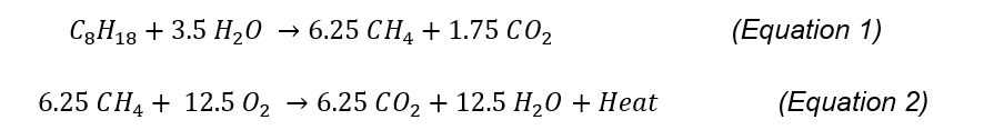
Most NAPL sources are methanogenic because external electron acceptors (i.e., sulfate or oxygen) are locally depleted and limited by transport from upstream groundwater sources (Lundegard and Johnson, 2005). Equation 1 represents the initial generation of biogas (a mixture of CH₄ and CO₂) upon methanogenic degradation of the NAPL contaminant. Equation 2 describes shallow methane oxidation upon contact with ambient oxygen diffusing downwards from the ground surface. Processes associated with Equations 1 and 2 occur at different depths of the soil column (anaerobic and aerobic, respectively). When combined, Equations 1 and 2 add up to an equation (Equation 3) characteristic of the entire NAPL-impacted soil column, from the ground surface to the deep contaminant location:

The basis for estimating NSZD rates is done by measuring the rate of production of reaction products (i.e., methane, CO₂, or heat) using either a mass balance or a heat balance. An additional method called the compositional change method, which tracks temporal changes in the composition of the remaining contaminant instead of the reaction products (Hostettler et al., 2013), will not be addressed here. Assuming octane (C₈H₁₈) as an example in Equations 1-3, a CO₂ flux of one micromole of CO₂ per square meter per second produced from the NAPL source results in an equivalence of 625 gallons of NAPL per acre per year of NAPL mass losses. Of course, a different formula weight characteristic of a specific site can be used instead of octane, which typically changes the equivalence by less than 10%.

To understand the variability of NSZD rates, it is useful to consider major factors affecting biodegradation rates. These major factors include:

1. Soil Temperature. Soil Temperature. Laboratory data suggests that for each 10˚C increase in soil temperature, microbial activity nearly doubles in the range between 0-40˚C. This increase in microbial activity may impact NSZD, although deeper soil temperatures, around 10 ft below ground surface or higher, are relatively stable (staying at the 15 to 16˚C range year-round). Furthermore, soil temperature will likely affect mass transfer rates (dissolution or volatilization) (Sookhak Lari et al., 2025).
2. NAPL distribution. NSZD processes are often mass transfer limited, meaning physical transport between the NAPL and surrounding phases is the rate-limiting step. Because mass transfer depends on surface area, broader distribution of NAPL in the soil column (referred to as the “smear zone”) will often result in larger NSZD rates because a larger portion of the soil microbiome can participate in the degradation mechanisms (Sookhak Lari et al., 2025).
3. NAPL composition. Microbial activity is selective towards some NAPL compounds over others (Hostettler et al., 2013). As the more biodegradable compounds are preferentially degraded, the NAPL source becomes enriched with less biodegradable (more recalcitrant) compounds, changing the NAPL composition and reducing the long-term NSZD rate. A study tracking long-term NSZD rates at a contaminated coastal petroleum handling site found that diesel NSZD rates were 3-6 times lower after 14 years, while gasoline NSZD rates were 9-27 times lower after a decade (Davis et al., 2022). Using initial NAPL mass estimates, the rates predicted total mass depletion by 2020, but mass measurements conducted that year still showed significant mass remaining (i.e., 25% of the initial gasoline still was accounted for).

Additional parameters might affect NSZD rates. For example, microbial activity requires minimal moisture levels and the presence of trace minerals and nutrients (e.g., nitrogen and phosphorus). However, the impact of these parameters on rates is poorly documented and thought to be minor at most sites. Therefore, a simplified NSZD conceptual model can be created by looking at the effects of the three above variables (soil temperature, NAPL distribution, and NAPL composition) to start analyzing general data trends.

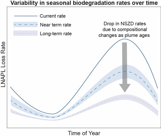
A “stylistic” mathematical model was developed by Zimbron (2016; et al., 2018) based on data from the Bemidji site to estimate the seasonal variability of NSZD rates, primarily accounting for temperature sensitivity. The model used inputs such as ambient temperature profiles and published contaminant distributions (Dillard et al., 1997) to calculate temperature-dependent degradation rates across the distribution of NAPL. The model predictions were calibrated by adjusting microbial degradation kinetics (obtained from a lab study using contaminated soils from a Canadian site at 22˚C) to match published measured bulk NSZD rates. These were collected at different times of the year at one location of the Bemidji site using background-corrected CO₂ fluxes measured with the dynamic closed chamber (Sihota, 2014). Note that this short-term variability will depend on many factors: depth to contamination, local ambient temperature fluctuations, groundwater temperature, etc. The annual rates depicted in Figure 1 represent a shallow, temperate site, but a site with more constant weather and/or deeper contamination might result in smaller seasonal NSZD rate variability.

These results illustrate that ambient temperature fluctuations can explain significant seasonal variability. In this case, the maximum annual NSZD rate might be up to four times the minimal rate. Furthermore, long-term reductions of these initial NSZD rates are likely to occur (in this case, using the results provided by the Davis et al., 2022 data).

3. The NSZD Signal and Its Measurement: Distinguishing Signal vs. Noise, and Signal Shredding

The previous section described a rough approximation of expected NSZD rates over the short term (one year) and long term (decades). An ideal NSZD measurement would generate similar data trends illustrated by Figure 1. In practice, each NSZD measurement method can introduce additional measurement errors that make the data trends even less clear. Two common sources of measurement error are noise and signal shredding. A case study illustrating these concepts will be presented in the next section.

3.1 Noise vs. Signal

The reaction products of NSZD shown in Equations 1-3 are also naturally produced by soils, associated with processes not related to contaminant NSZD, generating a “noise” in the measurement, while the signal related to the NSZD processes (the “NSZD signal”) plus the noise adding up to the total or unfiltered signal, according to Equation 4.

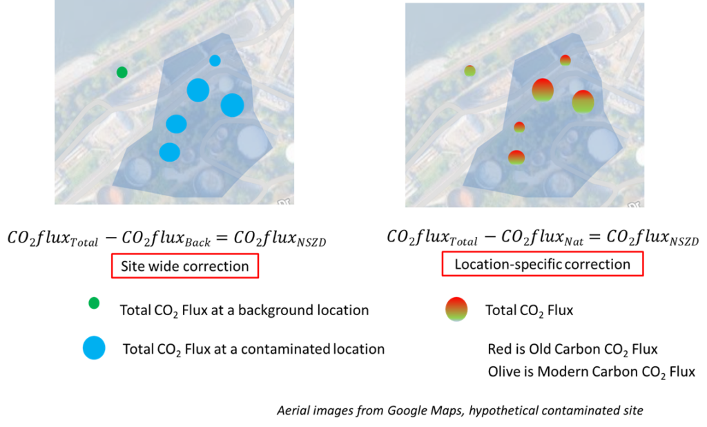
For example, uncontaminated soils naturally produce CO₂. Similarly, ambient temperature variations generate heat fluxes in soil that interfere with the heat flux of the biogenic heat from Equation 2. Different NSZD rate measurements deal with these interferences (the separation of signal from noise) in distinct ways. Figure 2 shows two different implementations of Equation 4. The first one is the so-called background location correction, in which a site-wide value is subtracted from the values obtained at the contaminated locations. For example, an NSZD rate measurement based on surficial CO₂ flux can be based on the total CO₂ flux, in which the total CO₂ flux at a background location (if available) is subtracted from the total CO₂ flux at the five contaminated locations shown. The second practice, not available for all methods, consists of applying a location-specific correction. When this occurs, the total CO₂ flux at each location can be calculated by using a radiocarbon (¹⁴C) analysis to differentiate the modern carbon CO₂ flux (noise) and the fossil fuel CO₂ flux (signal). The radiocarbon analysis has long been recognized as the most reliable correction (API, 2017; CRC Care, 2018). A study based on data from passive CO₂ traps found that the assumption of a single, site-wide value is rarely met and using it might result in large measurement error compared to the location-specific correction using the radiocarbon analysis (Zimbron, 2022).

3.2 Signal Shredding

Carbon dioxide, one of the main products of NSZD (Equation 3), is subject to gas transport between the location where it is generated to the location where it is measured. Similarly, the heat produced by NSZD (Equation 2) is subject to heat transport. Although the rate of these NSZD reactions might be nearly constant at the signal source over the short term (a few days or weeks), the reaction products will show up at the ground surface (or other discrete locations in soil chosen for measurement) at variable rates. For example, biogas (CH₄ and CO₂) produced by anaerobic digestion accumulates in the water phase (i.e., below the water table), forming bubbles. These bubbles grow until they are released episodically from saturated zones due to changes in ambient pressure and temperature in a process called ebullition. Furthermore, gas transport in the unsaturated zone (thought to occur mostly by diffusion), experiences an advective component near the surface caused by ambient pressure fluctuations (Ma et al., 2013). As a result, a NSZD process occurring at a nearly constant rate at the source will result in a variable expression at the location used to conduct the NSZD rate measurement. This effect has been referred to as “signal shredding” (Ramirez et al., 2015). Signal shredding is part of the reason why short-term total CO₂ fluxes from soils vary, following a diurnal sine-wave shape, indicating soil respiration rates can change and even reverse in the short term (Ma, et al., 2013).

The variability of soil property measurements and soil transport, and the added variability to soil transport caused by signal shredding, have been common problems facing soil scientists for a long time. For example, soil porosity measurements will depend on sample size. Large measurement variability will result if the sample volume is similar to the volume of a single particle (for example, using a spoon to obtain gravel samples). Increasing the sample size to the point that is larger than the particle size will result in measurements of soil porosity that are more consistent (have lower variability). The smallest scale at which the results no longer depend on the sample size is called the characteristic scale (or the minimum reference element volume). This broad concept applies not only to the properties of porous media, but also to soil transport processes (i.e., groundwater flow). For example, the characteristic scale of flow in porous media corresponds to the cube of the pore volume (Corey, 1994). In other words, the problem of variability in measurements caused by signal shredding can be addressed by sampling at a scale above the characteristic scale.

So far, the literature describing measurement methods for NSZD rates has lacked an explicit consideration of the characteristic scale. However, this concept and the distinction between signal and noise are key to understanding why results of NSZD rate measurements using different methods can be difficult to reconcile. Paraphrasing John Cherry, known as the father of groundwater contaminant hydrology, you know you have sufficient data when you throw away half of it and you reach similar conclusions (for a more in-depth discussion on this topic, see Cherry, 1990).

4. A Case Study Comparing Two Surficial Carbon Dioxide Flux-Based Methods

This publicly available case study (Malander et al., 2015) involves the use of two measurement techniques of NSZD rates based on surficial CO₂ fluxes: the dynamic closed chamber (DCC) and the passive CO₂ trap. This dataset is the only available case in which the DCC were deployed for an extended period (in this case the same deployment of the passive CO₂ trap, approximately 21 days), offering a unique opportunity to compare both techniques over the same deployment time. Although both methods intend to measure the NSZD rate using the soil CO₂ flux leaving the ground at the surface, they differ in two aspects: the time scale of the measurement, and how they handle the signal vs. noise correction. The DCC is intended to be a short-term measurement that measures the real-time build-up of CO₂, while the passive CO₂ trap uses a CO₂ sorbent to provide a long term, time-integrated measurement of the average total CO₂ flux during the period of deployment (typically 14 days). The passive CO₂ trap also uses a radiocarbon (¹⁴C) correction to differentiate the CO₂ of fossil fuel fraction (signal) from the modern carbon CO₂ captured (noise resulting from the natural carbon produced by soil respiration and decomposition). In contrast, the DCC often relies on subtracting the total CO₂ flux from a non-contaminated location (noise) from that of the total CO₂ flux measured at contaminated locations (noise + signal).

Due to the diurnal cycles in soil CO₂ gas caused by signal shredding, long-term use of the automated DCC is more rigorous than short-term DCC measurements for measuring NSZD rates. However, its practice might be limited to small NAPL-contaminated sites because automated DCC chambers need to be deployed within 50 feet of the CO₂ analyzer (a practical limitation imposed by the operating parameters of the sampling equipment involved). These practical limitations (and additional cost-related ones) in using the automated DCC makes this dataset unique and hard to replicate.

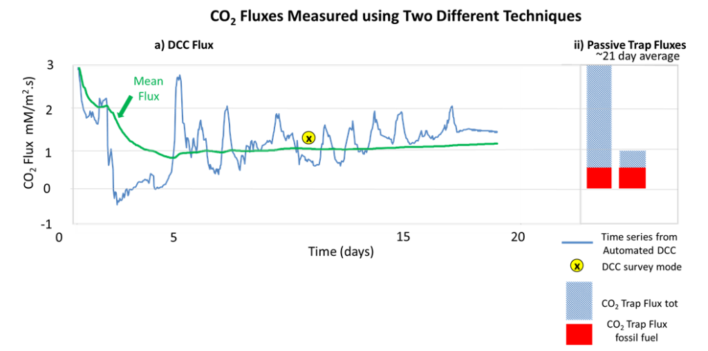
Figure 3 shows the time series of repeated DCC measurements for total CO₂ flux (in blue). Note that after the second day, the site experienced rain, which shut down the soil gas efflux, until the fifth day. At that point, a normal soil gas flux pattern (showing daily fluctuations) was reestablished. Figure 3 also shows the total CO₂ fluxes measured at two neighboring locations using the passive CO₂ traps, and the ¹⁴C-corrected data (used as the basis for the location-specific correction for NSZD rates with this technique) at both locations. The results show that the total CO₂ flux measured by the passive CO₂ traps were highly variable (although within the range of the time series measured by the DCC). However, the old carbon CO₂ flux (the ¹⁴C-corrected flux used to calculate NSZD rates) were within a few percentage points of each other with the measurement showing high repeatability. The time series from the DCC was used to calculate an average CO₂ flux up to that time shown in red. This data shows that the average soil gas flux of total CO₂ becomes nearly constant after 5 days. In other words, the characteristic scale of soil respiration process shown by this data set is around 5 days. Note that most DCC chamber measurements rely on a single time measurement and a background correction (also a single time measurement obtained at an uncontaminated location). Presumably, the total CO₂ flux at a background location would follow a daily pattern (as reported by Ma et al., 2013) and would have a characteristic scale of multiple days (as in Figure 3). Despite this short-term variability, practitioners have applied the ¹⁴C correction to single time DCC chamber measurements (for example, see Jourabchi et al., 2018 and Reynolds, 2021). In doing so, the benefits of the ¹⁴C high precision correction might be offset by the high variability of a measurement at a scale below the characteristic scale of the problem.

5. A Hypothetical Example

The example provided above is a detailed one, using real NSZD reported data. Here, a more general example will be provided for a hypothetical gas station, using an example provided before (Zimbron, 2025) involving a site (e.g., a gas station) with an existing mass of 32,000 gallons per acre. The initial analysis considered that at a NSZD rate of 700 gallons/acre/year (a mass loss rate of 2.2%), complete LNAPL depletion would be reached in approximately 30 years (ASTM, 2022). Now, consider that the stated rate was measured during the hottest part of the year, but a measurement during cold weather yields 300 gallons/acre/year, resulting in a reasonable annual average NSZD rate of 500 gallons/acre/year. If NAPL compositional changes resulted in lower NSZD rates over the long term by as much as an order of magnitude (as shown by Davis et al, 2022), then the life expectancy of the site can be easily pushed out in the future (by multiple decades). Whereas NSZD is expected to continue over the long term (at ever smaller rates), it would be wise to consider a range of life expectancy scenarios for the site, rather than a single value.

6. Summary and Recommendations

Differences in measured NSZD rates using multiple techniques can be difficult to reconcile, especially when the basis for these measurements is different. Many of the available methods are single time measurements (such as DCC), while others are time-integrated measurements (the passive CO₂ trap). The way that these measurements account for the sources of noise is also different. Some include a site-wide single value (the background location), while others use a location-specific value (for example the radiocarbon correction for CO₂ fluxes). Signal shredding and the lack of discussion about the characteristic scale of these processes create a very uneven field for these different techniques. No wonder practitioners have difficulty reconciling different measurement techniques. This should not be taken as a lack of repeatability of the methods themselves. For example, radiocarbon-corrected CO₂ fluxes using passive CO₂ trap data are within a few percentage points of each other (see Figure 3).

This document explains signal shredding and the distinction of noise vs. signal, which are two key drivers of variability in NSZD rate measurements, as illustrated for surficial CO₂ fluxes. However, additional sources of variability exist. A few examples are provided below:

Some methods measure gas concentrations or temperatures at discrete elevations in the soil column to calculate CO₂ fluxes or heat fluxes (i.e., the CO₂ gradient method or the thermal gradient method, respectively). These methods require the use of a soil transport property (i.e., the soil effective diffusion coefficient or the thermal diffusion coefficient, respectively). Often, practitioners will choose a single value from literature. The reported ranges of these coefficients often span over one order of magnitude. Furthermore, they will change with local soil conditions that rarely remain constant in time, such as soil type, moisture, and temperature. An inferred soil property from literature might differ from the actual (measured) one by orders of magnitude. An NSZD rate measurement obtained without measuring the actual soil properties, or one that is assumed to be constant over extended periods during which soil conditions vary will have large uncertainty.

The number of locations where NSZD is measured per unit area (the aerial sampling density) is another potential source of measurement error. A good practice here would be to pre-screen contaminated locations to define different levels of NSZD expression (i.e., high, medium, and low), over the entire contaminated area, and distribute sampling locations proportionally to the levels found during a pre-screening phase (stratified sampling).

NSZD rate measurements should ideally improve, not contradict, a conceptual site model (CSM). It might be tempting to discard NSZD rate measurements that do not fit the CSM. For example, background corrected CO₂ fluxes that are negative are often taken as null, but these should be taken as an indication that assumptions made while implementing the background correction were incorrect. Higher NSZD rates during colder weather, or the inverse, should be taken as a potential indication that the CSM needs further refinement or that the NSZD rate measurement is missing critical components of the CSM.

The CSM is unique to each site, and some sites have higher levels of complexity than others due to a variety of factors such as lithology, LNAPL distribution and site history. The risks associated with contamination are unique to each site, too. The suitability of NSZD as a remedy or as a reference for the performance of an active remedy will be site-specific. The practitioner must weigh these factors against the tolerance for uncertainty and the way that each method addresses measurement uncertainties before deciding on how to use NSZD rate data.

References

American Petroleum Institute. 2017. Quantification of Vapor Phase-Related Natural Source Zone Depletion Processes, First Edition. https://bit.ly/2Et9C43.

ASTM E3361-22, 2022. Standard Guide for Estimating Natural Attenuation Rates for Non-Aqueous Phase Liquids in the Subsurface. Last updated 12/12/2022.

Cherry, J.A., “Groundwater Monitoring: Some Deficiencies and Opportunities,” Hazardous Waste Site Investigations; Towards Better Decisions, Lewis Publishers, B.A. Berven & R.B. Gammage, Editors. Proceedings of the 10th ORNL Life Sciences Symposium, Gatlinburg, Tennessee, May 21–24 (1990). Available at: https://www.gfredlee.com/Groundwater/cherry_gw.pdf

Corey, A. 1994. Mechanics of Immiscible Fluids in Porous Media. Water Resources Publications.   

Craine, J. M., N. Fierer, K.K. McLauchlan, A.J. Elmore, Andrew J. 2013. Reduction of the temperature sensitivity of soil organic matter decomposition with sustained temperature increase. Biogeochemistry. 359- 368. 113 (1)

CRCCARE. 2018. Technical Measurement Guidance for LNAPL Natural Source Zone Depletion, CRCCARE Technical Report no. 44. Newcastle, Australia: CRC for Contamination Assessment and Remediation of the Environment.

Davis, G. B., J. L. Rayner, M.J. Donn, C.D. Johnston, R. Lukatelich, A. King, T.P. Bastow, and E. Bekele. 2022. Tracking NSZD mass removal rates over decades: Site-wide and local scale assessment of mass removal at a legacy petroleum site. Journal of Contaminant Hydrology. 248.

Dillard, L.A., H. I. Essaid, W. N. Herkelrath, and William N. Multiphase Flow Modeling of a Crude-Oil Spill Site With a Bimodal Permeability Distribution. Water Resource. Res. 33 (7). Pg. 1617-1632.

Hostettler, F.D., T. Lorenson and B.A. Bekins. 2013. Petroleum Fingerprinting with Organic Markers. Environmental Forensics .14(4). DO – 10.1080/15275922.2013.843611.

Jourabchi, P. A. Wozney, I. Hers, and H. Hopkins. 2018. Development of Protocol for Carbon Dioxide Efflux Measurements Using Dynamic Closed Chamber for NSZD Estimates. Battelle Chorinated Conference.

Kulkarni, P., K. L. Walker, C. J. Newell, K. K. Askarani, Y. Li, and T. E. McHugh. 2022. Natural Source Zone Depletion (NSZD) Insights From Over 15 Years of Research and Measurements: A Multi-Site Study. Volume 225, 15 October 2022, 119170. Water Research., 1-9.

Ma, J., Z. Wang, B. Stevenson, X. Zhen, and Y. Li. 2013.  An inorganic CO₂ diffusion and dissolution process explains negative CO₂ fluxes in saline/alkaline soils. Scientific Reports. 3(1).

Malander, M., H. Hopkins, A. Pennington, J. Smith, and S. Gaito. 2012. Comparison of Natural Source Zone Depletion Methods. Presented at 2012 International Petroleum Environmental Conference. Available at: https://cese.utulsa.edu/wp-content/uploads/2017/06/IPEC-2015-FIELD-COMPARISON-OF-NSZD-ASSESSMENT-METHODS-GRADIENT-METHOD-AND-TWO- CO₂-FLUX-METHODS-1.pdf

Ramirez, J.A., A.J.Baird, T.J. Coulthard, and  J.M. Waddington. 2015. Ebullition of Methane From Peatlands: Does Peat Act as a Signal Shredder? Geophysical Research Letters 42 : 3371 – 3379.    

Reynolds, L., U. Mayer, and I. Clark. 2018, Making Radiocarbon More Accessible for the Study of Biodegradation. Remediation Technologies Symposium. Banff, AB, Canada.

Sookhak Lari, K., Davis, G.B., and Rayner, J.L. A Roadmap to Understanding Key Knowledge Gaps in Natural Source Zone Depletion. Nat Water 3, 537–549 (2025). https://doi.org/10.1038/s44221-025-00436-5.

Zimbron, J. A. 2016. Establishment of Contaminant Degradation Rates in Soils Using Temperature Gradients, Associated Methods, Systems and Devices. U.S. Patent 10816441. Issued October 27, 2020.

Zimbron, J. A, J. DiMarzio, and G. Silco. 2018. Temperature Effects on Petroleum NSZD Processes: Lessons from Coupled Heat Transfer and Heat Generation Modeling. Battelle Chlorinated Conference, Palm Springs, CA. April 8-12.

Zimbron, J. A. 2022. Comparison of Radiocarbon- and Background Location-Corrections on Soil-Gas CO₂ Flux-Based NSZD Rate Measurements at Petroleum Impacted Sites. Groundwater Monitoring and Remediation. 116-122. 42 (23).

Zimbron, J. A. 2025. Resetting Expectations for the Rates of Natural Source Zone Depletion. LUSTLine, Issue 95.  NEWIPCC. Available at: https://neiwpcc.org/lustline/95/resetting-expectations-for-the-rates-of-natural-source-zone-depletion/